Image Optical Flow

Computes the optical flow from successive images.

Library

QUARC Targets/Image Processing/Generic

Description

The Image Optical Flow block computes the optical flow using successive images. It is similar to the Optical Flow block in the Computer Vision Toolbox, but may yield substantially better performance. Optical flow algorithms attempt to discern motion of the observer relative to the scene in successive images.

Consider two successive image frames where the intensity of the image at time t and pixel (x,y) is denoted by I(x,y,t). Optical flow algorithms assume the intensity does not change significantly between two successive frames i.e. that:

I(x + Δx, y + Δy, t + Δ) = I(x,y,t)

This constraint is called the brightness constancy constraint. For small movements:

I(x + Δx, y + Δy, t + Δ) ≅ I(x,y,t) + ∂I/∂x Δx + ∂I/∂y Δy + ∂I/∂t Δt

From these two equations:

∂I/∂x Δx + ∂I/∂y Δy + ∂I/∂t Δt = 0

Dividing by Δt and letting V_x = Δx / Δt and V_y = Δy / Δt:

∂I/∂x V_x + ∂I/∂y V_y + ∂I/∂t = 0

The partial derivatives of the image intensity may be computed, but there are two unknowns, V_x and V_y, and only one equation. Hence, a further constraint is needed to solve for the velocities at (x,y). All optical flow algorithms add an additional constraint in order to solve this equation.

The Image Optical Flow block currently supports two algorithms: a global optical flow algorithm and a feature-based algorithm.

The global algorithm outputs a single 2-DOF velocity estimate based on the difference between successive images. It is an algorithm based on the sum of absolute differences between images. It works best at higher sampling rates and lower image resolutions, although it is fast enough to be performed on higher resolution images as well. However, the higher the resolution, the faster the sample rate needs to be.

The feature-based algorithm is the pyramidal Lucas-Kanade algorithm. The Lucas-Kanade algorithm assumes the velocities of pixels in a local neighbourhood are the same to get more than one equation for the same V_x and V_y. Since any more than two pixels in this local neighbourhood makes the equations overconstrained, it uses a least squares estimation to solve for the pixel velocities. Since the standard Lucas-Kanade algorithm is generally only accurate for small displacements, this implementation uses a pyramidal version of the algorithm. This means that it applies the algorithm to successively downsampled versions of the image so that larger displacements can be detected.

Image pyramids are formed by taking an image and then filtering and downsampling it multiple times (filtering each time the image is downsampled). The resulting "stack" of images resembles a pyramid because each successive level has a smaller resolution. In the Image Optical Flow block, the image pyramid of successively downsampled images is formed according to three parameters: the number of pyramids, a pyramid rate and a separable, symmetric image kernel. The pyramid rate is the decimation factor to apply when downsampling from one level of the "pyramid" to the next. The image kernel is convoluted with each image prior to downsampling to filter each image. The downsampling takes every Nth pixel if the pyramid rate is an integer N. If a non-integral pyramid rate is specified then it uses bilinear interpolation to downsample the image.

The Image Optical Flow block implements a highly optimized version of the Lucas-Kanade algorithm for the target processor. For the Lucas-Kanade algorithm, the Image Optical Flow block currently supports only grayscale (HxW) uint8 images on the QUARC Win64 and QUARC Linux x64 targets. The global algorithm is supported on all targets.

Input Ports

image

The input is a MATLAB grayscale (HxW) uint8 image. The input is compatible with the MathWorks Computer Vision Toolbox.

Output Ports

points

For the feature-based algorithm, the output is a 2xN matrix of velocities, where N is the number of features selected in the dialog parameters. For the global algorithm it is 2-vector of velocity reflecting the overall velocity detected from successive images.

error

For the feature-based algorithm, the output is an N-vector, where N is the number of features selected in the dialog parameters. Each element is the RMS error between the old and new locations of the corresponding features based on the neighbourhoods. For the global algorithm it is scalar that is always zero (for now).

valid

For the feature-based algorithm, the output is an N-vector, where N is the number of features selected in the dialog parameters. Each element indicates the pyramid level at which the flow was determined. For the global algorithm it is scalar indicating whether the flow result is valid.

Parameters and Dialog Box

Main Pane

The Main pane of the dialog appears as follows:

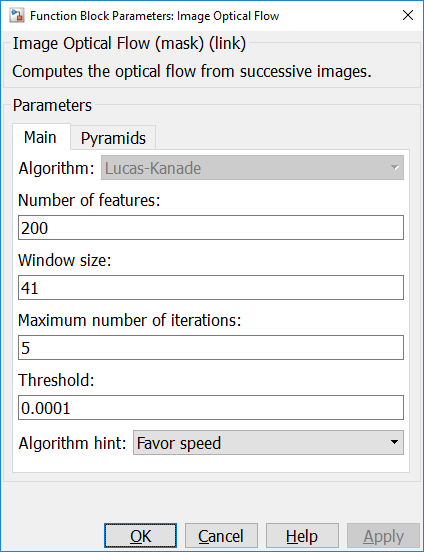
Type

The type of optical flow algorithm to use. Currently only the global or feature-based algorithms are supported, but future versions of this block are expected to support other types of algorithms.

Global Pane

The Global pane of the dialog appears as follows:

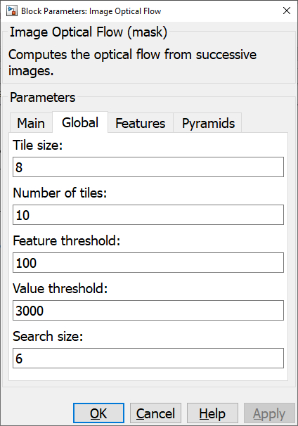
This tab only applies to global optical flow algorithms. Hence, it is only applicable when the optical flow Type parameter on the Main tab is equal to Global.

Tile size (tunable offline)

The size in pixels of the width and height of each tile used in determining the global optical flow.

Number of tiles (tunable offline)

The number of tiles to evaluate both horizontally and vertically in determining the global optical flow. While increasing the number of tiles does increase the computational overhead, the increase is typically less than expected because areas of the image which would not yield good optical flow results are quickly rejected and only those regions which are expected to yield good results are evaluated further.

Feature threshold (tunable offline)

The threshold to use in determining whether a region is suitable for optical flow determination. If the average pixel gradient horizontally and vertically within a tile is less than this threshold then the tile is rejected and not used for the optical flow determination.

Value threshold (tunable offline)

The threshold to use in determining whether a tile in the previous image matches a tile within the search distance in the new image. The sum of absolute differences between the two tiles must be less than this threshold.

Search size (tunable offline)

The maximum distance in pixels that a tile is expected to move from one image to the next. The speed of the algorithm is highly dependent on this parameter, so fast frame rates are ideal to ensure that this parameter may be small.

Features Pane

The Features pane of the dialog appears as follows:

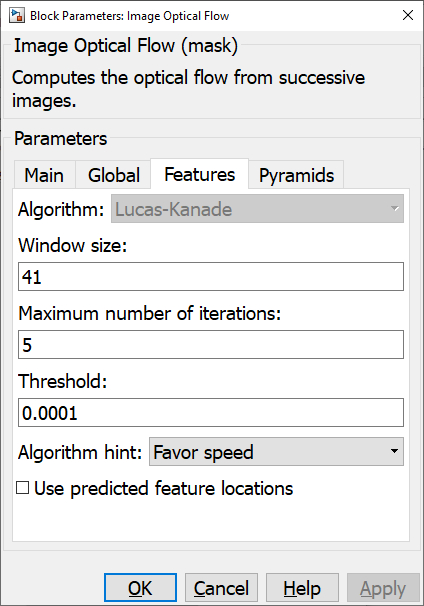
This tab only applies to feature-based optical flow algorithms. Hence, it is only applicable when the optical flow Type parameter on the Main tab is equal to Features.

Algorithm

The optical flow algorithm to use for feature-based optical flow. Only the Lucas-Kanade algorithm is currently supported, but future versions of this block are expected to support other algorithms.

Number of features

The number of features to track.

Window size (tunable offline)

The size of the search window to use.

Maximm number of iterations (tunable offline)

The maximum number of iterations to perform.

Threshold (tunable offline)

The threshold used for determining pixel movement. The larger the number the less small motions will impact the optical flow.

Algorithm hint (tunable offline)

Provides a hint to the algorithm as to whether it should favour speed or accuracy.

Pyramids Pane

The Pyramids pane of the dialog appears as follows:

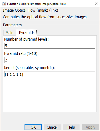
Number of pyramid levels (tunable offline)

The number of pyramid levels.

Pyramid rate (tunable offline)

The decimation factor from one level of the pyramid to the next. Valid values range from 1 to 10. Integer values do simple decimation. Non-integral values use bilinear interpolation.

Kernel (separable, symmetric) (tunable offline)

An odd-length vector representing a separable, symmetric kernel matrix that is convoluted with the image at each level prior to downsampling. The image kernel determines the filtering that is applied.

Targets

Copyright ©2024 Quanser Inc. This page was generated 2024-04-16. Submit feedback to Quanser about this page.

Link to this page.