PWM Output Configuration

QUARC allows PWM outputs to be configured in a variety of ways. This page describes the options available and the associated terminology. Most cards only provide a small subset of the available options, but some data acquisition cards, like the Quanser QPID, support almost all the options.

QUARC currently associates five primary characteristics with a PWM output:

• mode

• frequency

• configuration

• alignment

• polarity

PWM Mode

The PWM mode determines how the values written to the PWM output are interpreted. Under most circumstances, the duty cycle of the PWM output is modulated so that the period of the PWM pulse train is fixed but the duty cycle varies. This mode of operation is called PWM_DUTY_CYCLE_MODE (0) in QUARC. The full list of modes available is:

PWM_DUTY_CYCLE_MODE

In this mode, the duty cycle of the PWM pulses is varied when writing to the PWM outputs. This mode is suitable for most PWM applications, such as 3-phase motor control and driving RC servos. A sample pulse train with varying duty cycle is illustrated below.

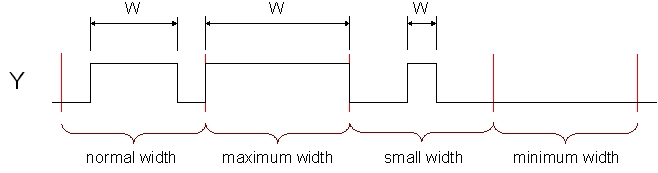
In the above example, the width of the pulse varies according to the duty cycle written to the PWM output. The red lines demarcate the PWM period. The period is determined by the PWM frequency programmed for the PWM output at initialization. For example, a PWM frequency of 10 kHz will yield a PWM period of 100 microseconds. This particular example uses center-aligned PWM so the pulse is centered within the PWM period.

For the relationship between PWM frequency and the effective number of bits in the PWM output, refer to the PWM Frequency section.

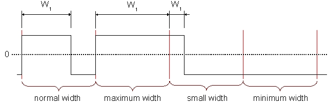
PWM_FREQUENCY_MODE

In this mode, the frequency of the PWM pulses is varied when writing to the PWM outputs while the duty cycle is maintained constant. This mode is rarely used but may be employed for frequency-modulation (FM) experiments or velocity control of stepper motors. An example of a PWM output in PWM_FREQUENCY_MODE is depicted below.

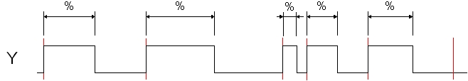
The red lines in the illustration delineate the PWM periods. The period varies with time as the PWM frequency is modulated by writing to the PWM outputs. Notice that the duty cycle of the pulse, however, remains the same. In this example, the duty cycle is 50%. Hence, the pulse width is always 50% of the PWM period, even as the PWM period varies.

PWM_PERIOD_MODE

This mode is analogous to the PWM_FREQUENCY_MODE. The only difference is that the PWM period is written to the PWM outputs rather than the frequency. The net effect is the same, but the signal used to drive the PWM outputs is the inverse of the frequency.

PWM_ONE_SHOT_MODE

This mode is analogous to the PWM_DUTY_CYCLE_MODE. The only difference is that only a single pulse is generated each time a value is written to the PWM outputs.

PWM_TIME_MODE

This mode is analogous to the PWM_DUTY_CYCLE_MODE. The only difference is that the width of the active PWM pulse in seconds is written to the PWM outputs rather than the duty cycle as a percentage. The net effect is the same, but the signal used to drive the PWM outputs is expresseed in seconds.

PWM_ENCODER_EMULATION_MODE

In this mode, the PWM outputs emulate the A and B signals of an encoder with full quadrature. To get both signals, the channels must be configured as paired or complementary outputs. Complementary outputs will produce an encoder output going in the opposite direction to paired outputs. If the output is configured as unipolar then only the A signal is generated.

The value written to the PWM outputs is the encoder velocity in counts per second. The PWM outputs will produce the same counts per second if connected to an encoder input supporting full 4X quadrature. The range of velocities is limited by the range of PWM frequencies supported by the card. A velocity of zero is generally always achievable.

The velocities may be positive or negative. The phase of the A and B signals is adjusted to account for the sign of the velocity. The PWM alignment setting is ignored in this mode because the phase relationship between the A and B signals must change dynamically with the sign of the velocity.

PWM Frequency

The PWM frequency determines the period of the pulses in the PWM output. It is important to understand the relationship between the PWM frequency and the PWM timebase. The PWM timebase is the clock used to generate the PWM output. It determines the minimum pulse width and therefore the effective resolution of the PWM signal.

For example, suppose the PWM timebase is 20 MHz. Hence, the minimum pulse width is 50 nanoseconds (1/20e6). If the PWM frequency is set to 10 kHz or 100 microseconds, then the effective resolution of the PWM signal is log2(100e-6 / 50e-9) = log2(2000) = 10.97 or approximately 11 bits. To get exactly N bits of resolution, set the PWM frequency to:

PWM frequency = PWM timebase frequency / (2N)

For example, to get 12 bit resolution when the PWM timebase is 20 MHz, use a PWM frequency of 20e6 / (212) = 4.882 kHz .

PWM Configuration

The PWM configuration determines the relationship between PWM outputs, if any. There are currently four PWM configurations possible:

PWM_UNIPOLAR_CONFIGURATION

In this configuration, the PWM output appears at a single output pin and is unipolar. For example, the output may vary between 0V and 3.3V. Some cards allow the input to be positive or negative, in which case the unipolar PWM output is switched between two output pins depending on the sign. This scenario is typically used when driving an H-bridge.

In the above example, the low value of the output is 0V and the high value is the digital V_cc. The duty cycle and period are determined by a single PWM channel. This particular example uses leading-edge alignment. For a discussion of all the different alignment options with the unipolar configuration, refer to the section on PWM Alignment.

PWM_BIPOLAR_CONFIGURATION

In this configuration, the PWM output appears at a single output pin and is bipolar. For example, the output may vary between -3.3V and 3.3V.

In the above example, the low value of the output is -V and the high value is V. The intermediate value is 0V. The magnitude, V, depends on the data acquistion card. The QPID card uses an analog output for bipolar PWM, so the magnitude of the output is determined by the last value written to the corresponding analog output channel.

The value of the output is determined by two PWM channels. The first, or primary, PWM channel controls the width of the high pulse and the second, or secondary, PWM channel controls the width of the low pulse. The primary channel is typically an even-numbered channel, and the secondary channel is generally the next odd-numbered channel. The deadbands determine the distance between pulses. This particular example uses leading-edge alignment. For a discussion of all the different alignment options with the bipolar configuration, refer to the section on PWM Alignment.

On the QPID card, the first four analog outputs are used for bipolar PWM. For any output to appear, write a non-zero value to the appropriate analog output channel. The bipolar PWM signal will then modulate that amplitude. The amplitude may be changed at any time by writing a new value to the analog output.

The table below shows the relationship between the analog output channels and the corresponding PWM channels in bipolar mode for the QPID card.

PWM_PAIRED_CONFIGURATION

In this configuration, the PWM output appears at two output pins: a primary output and a secondary output. The secondary output is a reflection of the primary output, except that deadband may be added between the rising and falling edges of the outputs. The paired configuration may be used for 3-phase motor control and other applications where series transistors are being switched on and off by the PWM signals.

In the above example, the red lines demarcate the PWM period. This particular example uses leading-edge alignment. For a discussion of all the different alignment options with the paired configuration, refer to the section on PWM Alignment.

The width of the primary output, Y₁, is determined by the duty cycle set for the corresponding PWM channel. This width is reduced by the leading-edge deadband, L, to ensure that the secondary output, Y₂, never switches at the same time. However, this deadband may be set to zero. The secondary output falls T seconds after the falling edge of the primary output, where T is the trailing-edge deadband. This deadband may also be set to zero. Note that the width of the primary pulse can never be larger than the PWM period minus the sum of the deadbands to ensure that the deadband is always maintained between the edges of the primary and secondary outputs - even if the duty cycle is continually varying i.e., the time between edges across PWM periods must be considered, not just the time between edges within a PWM period.

The figure illustrates how the two paired outputs behave for a variety of duty cycles, from the smallest to the largest. Note that the primary output goes to zero once the pulse width falls below the leading-edge deadband.

When using the paired configuration, the settings for the secondary PWM channel are ignored. However, they should be set to the unipolar configuration with leading-edge alignment and active-high polarity. This proviso is particularly important in Simulink, since the HIL Initialize block would take a PWM configuration vector of [2], indicating the paired configuration, and assign every PWM channel in the PWM Channels list the paired configuration. However, if a PWM configuration vector of [2 0] is specified, then it assigns the paired configuration to the first PWM channel in the list and the unipolar configuration to all subsequent channels.

PWM_COMPLEMENTARY_CONFIGURATION

In this configuration, the PWM output appears at two output pins: a primary output and a secondary output. The secondary output is the inverse of the primary output, except that deadband may be added between the rising and falling edges of the outputs. The paired configuration may be used for 3-phase motor control and other applications where series transistors are being switched on and off by the PWM signals.

In the above example, the red lines demarcate the PWM period. This particular example uses leading-edge alignment. For a discussion of all the different alignment options with the complementary configuration, refer to the section on PWM Alignment.

The width of the primary output, Y₁, is determined by the duty cycle set for the corresponding PWM channel. This width is reduced by the leading-edge deadband, L, to ensure that the secondary output, Y₂, never switches at the same time. However, this deadband may be set to zero. The secondary output rises T seconds after the falling edge of the primary output, where T is the trailing-edge deadband. This deadband may also be set to zero. Note that the width of the primary pulse can never be larger than the PWM period minus the sum of the deadbands to ensure that the deadband is always maintained between the edges of the primary and secondary outputs - even if the duty cycle is continually varying i.e., the time between edges across PWM periods must be considered, not just the time between edges within a PWM period.

The figure illustrates how the two complementary outputs behave for a variety of duty cycles, from the smallest to the largest. Note that the primary output goes to zero once the pulse width falls below the leading-edge deadband.

When using the complementary configuration, the settings for the secondary PWM channel are ignored. However, they should be set to the unipolar configuration with leading-edge alignment and active-high polarity. This proviso is particularly important in Simulink, since the HIL Initialize block would take a PWM configuration vector of [3], indicating the complementary configuration, and assign every PWM channel in the PWM Channels list the complementary configuration. However, if a PWM configuration vector of [3 0] is specified, then it assigns the complementary configuration to the first PWM channel in the list and the unipolar configuration to all subsequent channels.

PWM Alignment

The alignment determines how the pulse is aligned within the PWM period. There are three types of alignment, as shown in the following table.

These alignment options are described for each possible PWM configuration below. Only PWM_DUTY_CYCLE_MODE is discussed because it is the only mode currently supported for all the different PWM configurations.

PWM_LEADING_EDGE_ALIGNED

In leading-edge alignment, the pulse is aligned to the leading-edge of the PWM period. Regardless of the PWM configuration, such alignment means that the leading edge of the pulse always occurs at the same point relative to the beginning of the PWM period, while the trailing edge of the pulse varies according to the duty cycle.

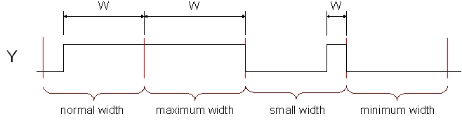
Leading-Edge Aligned, Unipolar PWM

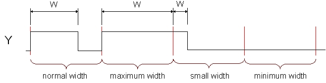
The following figure illustrates leading-edge alignment in the unipolar configuration.

The red lines demarcate the PWM period. Notice that the leading, or rising edge, of the PWM pulse always occurs at the beginning of the PWM period. The width of the pulse, w, is determined by the duty cycle of the PWM channel. As the duty cycle varies, the width of the pulse changes but the rising edge of the pulse always occurs at the start of the PWM period. The falling edge varies with the duty cycle. At 100% duty cycle, the PWM output is always high and at 0% duty cycle the output is always low.

Leading-Edge Aligned, Bipolar PWM

This next figure depicts leading-edge alignment in the bipolar configuration.

The red lines demarcate the PWM period. The width of the high pulse, w1 , is determined by the duty cycle of the primary PWM channel, and the width of the low pulse, w2 , is set by the duty cycle of the secondary PWM channel.

If the leading-edge deadband, L, is zero, then the leading, or rising, edge of the high pulse is always aligned to the start of the PWM period when leading-edge alignment is used. In this particular example, the leading-edge deadband is non-zero. Hence, the width of the high pulse is reduced by the leading-edge deadband. Therefore, the high pulse occurs at a fixed offset, L, from the start of the PWM period. This offset does not change as the duty cycle varies, so the rising edge of the high pulse always occurs at the same time within the PWM period. The falling edge of the high pulse, on the other hand, does vary with the duty cycle. If the duty cycle of the primary channel falls below the leading-edge deadband then the high pulse goes to zero.

The low pulse always begins T seconds after the falling edge of the high pulse, where T is the trailing-edge deadband. This deadband may be zero, in which case the falling edge of the high pulse and the start of the low pulse coincide. Notice that the width of the low pulse is reduced by the trailing-edge deadband, much like the high pulse is reduced by the leading-edge deadband. If the duty cycle of the secondary channel falls below the trailing-edge deadband then the low pulse goes to zero.

If the sum of the two duty cycles exceeds 100% then the width of the low pulse is reduced to ensure the sum of the duty cycles is never more than 100%. This supremacy of the primary channel may be used to advantage. For example, if the duty cycle of the secondary channel is set to a constant 100% and the deadbands are set to zero, then the bipolar output illustrated below may be generated.

Notice that the signal now varies between -V and +V and never goes to zero. The width of the pulse is determined solely by the duty cycle of the primary PWM channel in this case, and the pulse is aligned to the start of the PWM period. Thus, the output looks just like a unipolar PWM output except that the low value is not zero, but -V.

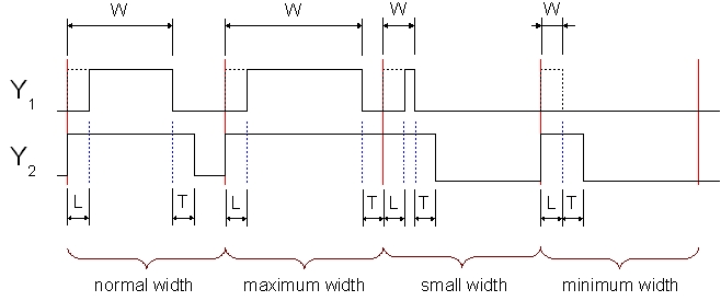
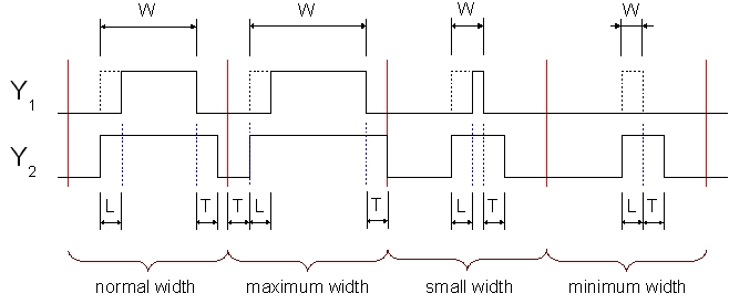
Leading-Edge Aligned, Paired PWM

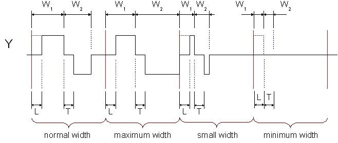
The following figure illustrates leading-edge alignment in the paired configuration.

The red lines demarcate the PWM period. Notice that the leading edge, or rising edge, of the secondary PWM pulse, Y₂, always occurs at the beginning of the PWM period when leading-edge alignment is employed. The width of the primary pulse, w, is determined by the duty cycle of the primary PWM channel. This width is reduced by the leading-edge deadband, L, to ensure that there is always at least L seconds between the rising edge of the secondary pulse and the rising edge of the primary pulse. The leading-edge deadband may be zero so that the two edges coincide. As the duty cycle varies, the widths of the two pulses change but the rising edge of the secondary pulse always occurs at the start of the PWM period, and the rising edge of the primary pulse is always delayed by the leading-edge deadband.

The falling edge of the secondary pulse always occurs T seconds after the falling edge of the primary pulse, Y₁, where T is the trailing-edge deadband. This deadband may be zero such that the two edges coincide. Since the falling edge of the secondary pulse is always a fixed offset from the falling edge of the primary pulse, the width of both pulses is determined by the duty cycle of the primary channel and the duty cycle written to the secondary PWM channel is ignored.

If the duty cycle of the primary PWM channel is less than the leading-edge deadband, L, then the primary output goes to zero. The secondary output does not go to zero, however, unless both deadbands are zero. There will always be a pulse on the secondary output that is at least as wide as the sum of the deadbands to guarantee that the deadbands are maintained, even across PWM periods. For the same reason, the primary output will never be always high unless the deadbands are both zero. It will always be limited to being low for at least the sum of the deadbands.

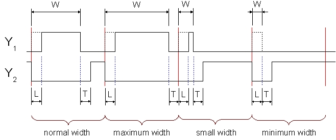
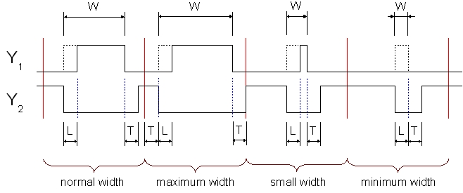
Leading-Edge Aligned, Complementary PWM

The figure below depicts leading-edge alignment in the complementary configuration.

The red lines demarcate the PWM period. Notice that the falling edge of the secondary PWM pulse, Y₂, always occurs at the beginning of the PWM period when leading-edge alignment is employed. The width of the primary pulse, w, is determined by the duty cycle of the primary PWM channel. This width is reduced by the leading-edge deadband, L, to ensure that there is always at least L seconds between the falling edge of the secondary pulse and the rising edge of the primary pulse. The leading-edge deadband may be zero so that the two edges coincide. As the duty cycle varies, the widths of the two pulses change but the falling edge of the secondary pulse always occurs at the start of the PWM period, and the rising edge of the primary pulse is always delayed by the leading-edge deadband.

The rising edge of the secondary pulse always occurs T seconds after the falling edge of the primary pulse, Y₁, where T is the trailing-edge deadband. This deadband may be zero such that the two edges coincide. Since the rising edge of the secondary pulse is always a fixed offset from the falling edge of the primary pulse, the width of both pulses is determined by the duty cycle of the primary channel and the duty cycle written to the secondary PWM channel is ignored.

If the duty cycle of the primary PWM channel is less than the leading-edge deadband, L, then the primary output goes to zero. The secondary output does not go completely high, however, unless both deadbands are zero. There will always be a low pulse on the secondary output that is at least as wide as the sum of the deadbands to guarantee that the deadbands are maintained, even across PWM periods. For the same reason, the primary output will never be always high unless the deadbands are both zero. It will always be limited to being low for at least the sum of the deadbands.

PWM_TRAILING_EDGE_ALIGNED

In trailing-edge alignment, the pulse is aligned to the trailing-edge of the PWM period. Regardless of the PWM configuration, such alignment means that the trailing edge of the pulse always occurs at the same point relative to the end of the PWM period, while the leading edge of the pulse varies according to the duty cycle.

Trialing-Edge Aligned, Unipolar PWM

The following figure illustrates trailing-edge alignment in the unipolar configuration.

The red lines demarcate the PWM period. Notice that the trailing, or falling edge, of the PWM pulse always occurs at the end of the PWM period. The width of the pulse, w, is determined by the duty cycle of the PWM channel. As the duty cycle varies, the width of the pulse changes but the trailing edge of the pulse always occurs at the end of the PWM period. The rising edge varies with the duty cycle. At 100% duty cycle, the PWM output is always high and at 0% duty cycle the output is always low.

Trailing-Edge Aligned, Bipolar PWM

This next figure depicts trailing-edge alignment in the bipolar configuration.

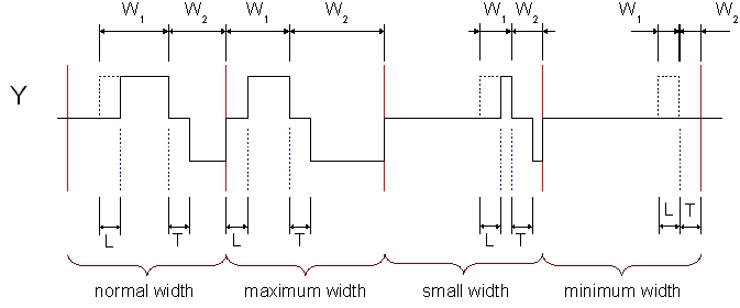
The red lines demarcate the PWM period. The width of the high pulse, w1 , is determined by the duty cycle of the primary PWM channel, and the width of the low pulse, w2 , is set by the duty cycle of the secondary PWM channel.

The trailing edge of the low pulse is always aligned to the end of the PWM period when using trailing-edge alignment, regardless of the duty cycle or deadbands. The leading edge of the low pulse varies with the duty cycle of the secondary PWM channel. The width of the low pulse is reduced by the trailing-edge deadband. If the width of the low pulse is less than the trailing-edge deadband, then the low pulse goes to zero.

The falling edge of the high pulse is always coincident with the leading edge of the low pulse if the trailing edge deadband is zero. Otherwise, there are T seconds between the two edges, where T is the trailing edge deadband.

The width of the high pulse is reduced by the leading-edge deadband, L. If the width is less than the leading-edge deadband then the high pulse goes to zero.

If the sum of the two duty cycles exceeds 100% then the width of the low pulse is reduced to ensure the sum of the duty cycles is never more than 100%.

Trailing-Edge Aligned, Paired PWM

The following figure illustrates trailing-edge alignment in the paired configuration.

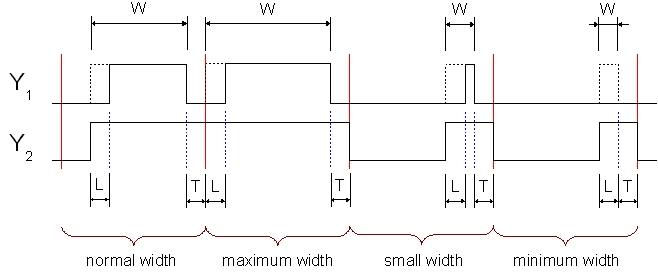
The red lines demarcate the PWM period. Notice that the trailing edge, or falling edge, of the secondary PWM pulse, Y₂, always occurs at the end of the PWM period when trailing-edge alignment is employed. The width of the primary pulse, w, is determined by the duty cycle of the primary PWM channel. This width is reduced by the leading-edge deadband, L, to ensure that there is always at least L seconds between the rising edge of the secondary pulse and the rising edge of the primary pulse. The leading-edge deadband may be zero so that the two edges coincide. As the duty cycle varies, the widths of the two pulses change but the falling edge of the secondary pulse always occurs at the end of the PWM period, and the rising edge of the primary pulse is always delayed by the leading-edge deadband.

The falling edge of the primary pulse, Y₁, always occurs T seconds before the falling edge of the secondary pulse, where T is the trailing-edge deadband. This deadband may be zero such that the two edges coincide. Since the falling edge of the primary pulse is always a fixed offset from the falling edge of the secondary pulse, the width of both pulses is determined by the duty cycle of the primary channel and the duty cycle written to the secondary PWM channel is ignored.

If the duty cycle of the primary PWM channel is less than the leading-edge deadband, L, then the primary output goes to zero. The secondary output does not go to zero, however, unless both deadbands are zero. There will always be a pulse on the secondary output that is at least as wide as the sum of the deadbands to guarantee that the deadbands are maintained, even across PWM periods. For the same reason, the primary output will never be always high unless the deadbands are both zero. It will always be limited to being low for at least the sum of the deadbands.

Trailing-Edge Aligned, Complementary PWM

The figure below depicts trailing-edge alignment in the complementary configuration.

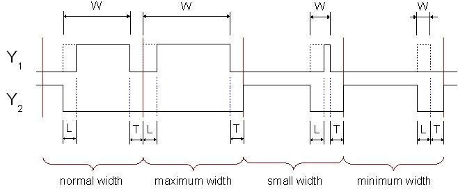
The red lines demarcate the PWM period. The secondary output, Y₂, is the inverse of the primary output, Y₁, because of the complementary configuration. Notice that the rising edge, of the secondary PWM pulse always occurs at the end of the PWM period when trailing-edge alignment is employed. The width of the primary pulse, w, is determined by the duty cycle of the primary PWM channel. This width is reduced by the leading-edge deadband, L, to ensure that there is always at least L seconds between the falling edge of the secondary pulse and the rising edge of the primary pulse. The leading-edge deadband may be zero so that the two edges coincide. As the duty cycle varies, the widths of the two pulses change but the rising edge of the secondary pulse always occurs at the end of the PWM period, and the rising edge of the primary pulse is always delayed by the leading-edge deadband.

The falling edge of the primary pulse, Y₁, always occurs T seconds before the rising edge of the secondary pulse, where T is the trailing-edge deadband. This deadband may be zero such that the two edges coincide. Since the falling edge of the primary pulse is always a fixed offset from the rising edge of the secondary pulse, the width of both pulses is determined by the duty cycle of the primary channel and the duty cycle written to the secondary PWM channel is ignored.

If the duty cycle of the primary PWM channel is less than the leading-edge deadband, L, then the primary output goes to zero. The secondary output does not go high, however, unless both deadbands are zero. There will always be a low pulse on the secondary output that is at least as wide as the sum of the deadbands to guarantee that the deadbands are maintained, even across PWM periods. For the same reason, the primary output will never be always high unless the deadbands are both zero. It will always be limited to being low for at least the sum of the deadbands.

PWM_CENTER_ALIGNED

In center alignment, the pulse is aligned to the middle of the PWM period. Thus, unlike the leading and trailing-edge alignments, the position of the leading and trailing edges of the pulses varies within the PWM period as the duty cycle varies.

Center Aligned, Unipolar PWM

The following figure illustrates center alignment in the unipolar configuration.

The red lines demarcate the PWM period. Notice that the PWM pulse always occurs in the middle of the PWM period. The width of the pulse, w, is determined by the duty cycle of the PWM channel. As the duty cycle varies, the width of the pulse changes but the pulse always remains centered within the PWM period. Hence, both the rising and falling edges vary with the duty cycle. At 100% duty cycle, the PWM output is always high and at 0% duty cycle the output is always low.

Center Aligned, Bipolar PWM

This next figure depicts center alignment in the bipolar configuration.

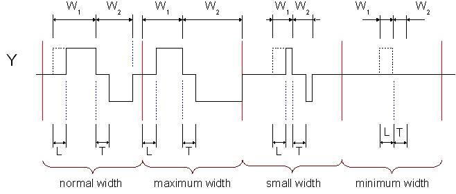
The red lines demarcate the PWM period. The width of the high pulse, w1 , is determined by the duty cycle of the primary PWM channel, and the width of the low pulse, w2 , is set by the duty cycle of the secondary PWM channel.

In this case, the high and low pulse sequence is centered within the PWM period based on the combined width w1 + w2. The leading-edge deadband, L, and trailing-edge deadband, T, are not taken into account when centering the pulses. However, the width of the high pulse is reduced by the leading-edge deadband, and the width of the low pulse is reduced by the trailing-edge deadband, to ensure that there is always a fixed deadband between edges. Either deadband may be set to zero so that the corresponding edges coincide.

As the duty cycles are varied, the widths of the pulses will vary accordingly and the pulse sequence will shift within the PWM period to remain centered. If the duty cycle of the primary PWM channel falls below the leading-edge deadband, L, then the high pulse goes to zero. If the duty cycle of the secondary channel falls below the trailing-edge deadband, T, then the low pulse goes to zero.

If the sum of the two duty cycles exceeds 100% then the width of the low pulse is reduced to ensure the sum of the duty cycles is never more than 100%.

Center Aligned, Paired PWM

The following figure illustrates center alignment in the paired configuration.

The red lines demarcate the PWM period. If the leading-edge deadband, L, is zero, then the primary output, Y₁, will always be centered within the PWM period. If the leading-edge deadband is non-zero, as shown, then the width of the primary pulse is reduced by the amount of deadband.

The secondary pulse, Y₂, is a reflection of the primary pulse, except for the deadband. The falling edge of the secondary pulse occurs T seconds after the falling edge of the primary pulse, where T is the trailing-edge deadband, and the rising edge of the secondary pulse occurs L seconds prior to the rising edge of the primary pulse, where L is the leading-edge deadband. The deadbands ensure that the two pulses do not switch at the same time, although either deadband may be set to zero. In that case, the corresponding edges would coincide.

The width of both pulses varies according to the duty cycle of the primary PWM channel. The duty cycle of the secondary PWM channel is ignored. If the duty cycle of the primary PWM channel is less than the leading-edge deadband, L, then the primary output goes to zero. The secondary output does not go to zero, however, unless both deadbands are zero. There will always be a pulse on the secondary output that is at least as wide as the sum of the deadbands to guarantee that the deadbands are maintained, even across PWM periods. For the same reason, the primary output will never be always high unless the deadbands are both zero. It will always be limited to being low for at least 2*T + L seconds.

Center Aligned, Complementary PWM

The following figure illustrates center alignment in the complementary configuration.

The red lines demarcate the PWM period. If the leading-edge deadband, L, is zero, then the primary output, Y₁, will always be centered within the PWM period. If the leading-edge deadband is non-zero, as shown, then the width of the primary pulse is reduced by the amount of deadband.

The secondary pulse, Y₂, is the inverse of the primary pulse, except for the deadband. The rising edge of the secondary pulse occurs T seconds after the falling edge of the primary pulse, where T is the trailing-edge deadband, and the falling edge of the secondary pulse occurs L seconds prior to the rising edge of the primary pulse, where L is the leading-edge deadband. The deadbands ensure that the two pulses do not switch at the same time, although either deadband may be set to zero. In that case, the corresponding edges would coincide.

The width of both pulses varies according to the duty cycle of the primary PWM channel. The duty cycle of the secondary PWM channel is ignored. If the duty cycle of the primary PWM channel is less than the leading-edge deadband, L, then the primary output goes to zero. The secondary output does not go high, however, unless both deadbands are zero. There will always be a low pulse on the secondary output that is at least as wide as the sum of the deadbands to guarantee that the deadbands are maintained, even across PWM periods. For the same reason, the primary output will never be always high unless the deadbands are both zero. It will always be limited to being low for at least 2*T + L seconds.

PWM Polarity

The PWM polarity is simply whether the output is active-high or active-low. In the paired and complementary configurations, the polarity of the secondary PWM output is determined by the polarity of the primary PWM channel.

Copyright ©2024 Quanser Inc. This page was generated 2024-04-16. Submit feedback to Quanser about this page.

Link to this page.