QUARC Dynamic Reconfiguration Demo

quarc_dynamic_reconfiguration_demo_model_1.mdl

quarc_dynamic_reconfiguration_demo_model_2.mdl; quarc_dynamic_reconfiguration_demo_supervisor.mdl

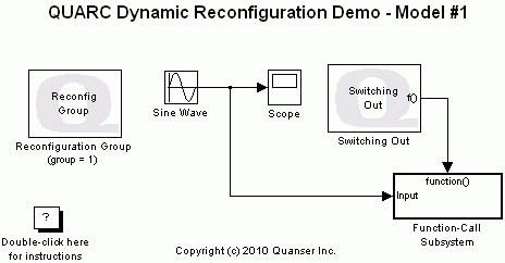
This example uses three Simulink models to demonstrate how to perform dynamic reconfiguration. For a detailed description of this feature, the models used and how they operate, please refer to the Dynamic Reconfiguration section of the QUARC documentation.

Dynamic Reconfiguration Demo Simulink Diagram

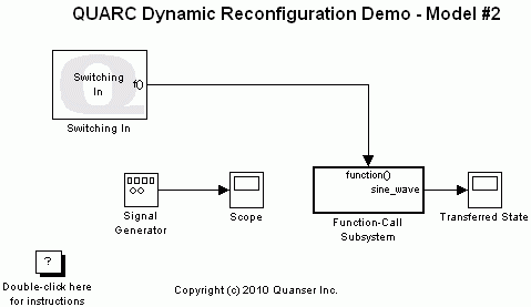
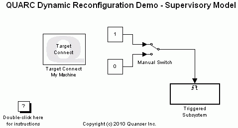
This demonstration consists of three sections; in the first section, simulating the dynamic reconfiguration process is demonstrated. Second section is dedicated to showcasing how to perform dynamic reconfiguration using a QUARC MATLAB function. The last section provides steps on performing dynamic reconfiguration using a supervisory model.

Note:

You need to have the proper license to run this demo. The dynamic reconfiguration feature support should be included in your QUARC license.

Configuring the Demonstration

To set up the demonstration, open the Configuration Parameters dialog box for the quarc_dynamic_reconfiguration_demo_model_1.mdl model by either pressing Ctrl+E or selecting the Model Settings button on the MODELING tab. Under the Code Generation/QUARC pane, make sure the Support dynamic reconfiguration parameter is enabled by clicking on its check box. Next, make sure that the MEX-file arguments parameter found under the Code Generation/Interface pane does not contain the "-w" option. If the "-w" option is included, delete it from the model arguments. For details about the reason for excluding this option, you can refer to the Creating Models to Support Dynamic Reconfiguration section. Repeat the same procedure for the quarc_dynamic_reconfiguration_demo_model_2.mdl model. For the third section of this demonstration, we use the quarc_dynamic_reconfiguration_demo_supervisor.mdl model. To setup this model for the third section, open the Triggered Subsystem and double-click on the Target Switch block. In the block parameters dialog, make sure the Name of model to switch in parameter is set to the name of the second model ("quarc_dynamic_reconfiguration_demo_model_2").

Demonstration 1 - Simulating Dynamic Reconfiguration

This demonstration illustrates how to simulate dynamic reconfiguration in normal simulation.

Make sure both quarc_dynamic_reconfiguration_demo_model_1.mdl and quarc_dynamic_reconfiguration_demo_model_2.mdl models have the SIMULATION tab selected.

Double-click on the Scope block in the quarc_dynamic_reconfiguration_demo_model_1.mdl model to display the sine wave on the scope. Double-click on the "Transferred State" block in the quarc_dynamic_reconfiguration_demo_model_2.mdl model.

Start the quarc_dynamic_reconfiguration_demo_model_1.mdl model's simulation by pressing Ctrl+T or clicking the Run button.

While model #1 is running, enter the following command in the MATLAB command window:

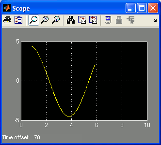
At this point, model #1 is dynamically switched out and model #2 is switched in. In other words, model #1 is stopped and model #2 starts running in normal mode. If you look at the scopes, you will notice that the "Transferred Data" scope is displaying a constant value (you might have to Autoscale the scope). This value corresponds to the value of the sine wave at the time the dynamic reconfiguration occurred multiplied by a value of 10. You can check the last value of the sine wave on the Scope block of model #1.

Model #1 Scope

Model #2 Scope

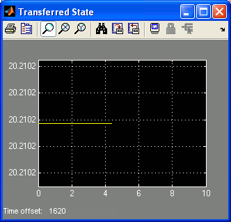
Stop model #2 simulation by pressing Ctrl+Shift+T or clicking the Stop button.

Demonstration 2 - Dynamic Reconfiguration Using the MATLAB Command Window

This demonstration illustrates how to perform dynamic reconfiguration using the MATLAB command window.

Make sure both quarc_dynamic_reconfiguration_demo_model_1.mdl and quarc_dynamic_reconfiguration_demo_model_2.mdl models have the HARDWARE tab selected.

Refer to One Step Process in QUARC Basic Procedures to build, deploy and start each model.

While model #1 is running, enter the following command in the MATLAB command window:

qc_switch_to_model('quarc_dynamic_reconfiguration_demo_model_2', 1);

At this point, model #1 is dynamically switched out and model #2 is switched in. In other words, model #1 is stopped and model #2 starts running in real-time. If you look at the scopes, you will notice that the "Transferred Data" scope is displaying a constant value (you might have to Autoscale the scope). This value corresponds to the value of the sine wave at the time the dynamic reconfiguration occurred multiplied by a value of 10. You can check the last value of the sine wave on the Scope block of model #1.

Model #1 Scope

Model #2 Scope

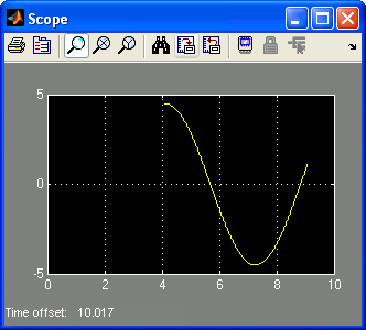
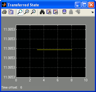
Refer to One Step Process in QUARC Basic Procedures to stop each model.

Demonstration 3 - Dynamic Reconfiguration Using a Supervisory Model

This demonstration illustrates how to perform dynamic reconfiguration using a supervisory model.

Make sure all of quarc_dynamic_reconfiguration_demo_model_1.mdl, quarc_dynamic_reconfiguration_demo_model_2.mdl and quarc_dynamic_reconfiguration_demo_supervisor.mdl models have the HARDWARE tab selected.

Refer to One Step Process in QUARC Basic Procedures to build, deploy and start each model.

While model #1 is running, double click on the Manual Switch block in the supervisory model to trigger the Triggered Subsystem.

At this point, model #1 is dynamically switched out and model #2 is switched in by the supervisory model. In other words, model #1 is stopped and model #2 starts running in real-time. If you look at the scopes, you will notice that the "Transferred Data" scope is displaying a constant value (you might have to Autoscale the scope). This value corresponds to the value of the sine wave at the time the dynamic reconfiguration occurred multiplied by a value of 10. You can check the last value of the sine wave on the Scope block of model #1.

Model #1 Scope

Model #2 Scope

Refer to One Step Process in QUARC Basic Procedures to stop each model.

Running the example on a different target

To run the example on a different target, refer to the instructions on the Running QUARC Examples on Remote Targets page.

Note that each model will require a different model URI since each model cannot use the same port.