MATLAB Command Line
Click to copy the following command line to the clipboard. Then paste it in the MATLAB Command Window:
quarc_multirate_demoQUARC Multi-Rate Demo
This example demonstrates the ability of QUARC to run multi-rate models in multiple threads. This capability ensures correct execution of the base rate and subrate tasks. The example highlights the difference between using a single thread to execute a multi-rate model versus multiple threads. The example model has two rates: a 100 Hz base rate and a slower 10 Hz subrate. A 1 kHz base rate is not used so that the example may be run on slower targets, such as the gumstix Verdex target. Of particular note is the use of a PI controller to moderate the computation time of the subrate task such that it takes 60 ms to execute on all targets. For details of QUARC's multi-rate capabilities, please refer to the Multithreading page in the QUARC documentation.
The red blocks in the model are configured to run at the base rate of 100 Hz. The green blocks
run at the subrate of 10 Hz. The sample time is configured by double-clicking on a source block
and setting the Sample time parameter to the desired sample time
in seconds. For the base rate, the QUARC function qc_get_step_size" may be
used, which returns the fixed step size configured for the model.
For example, double-click on the Repeating Sequence Stair block to open its parameters dialog.
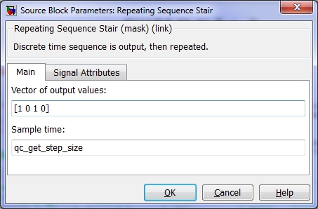
The Sample time parameter has been set to qc_get_step_size"
because this block should belong to the fast rate task.
On the other hand, double-click on the Computation Time block to open its parameters dialog.
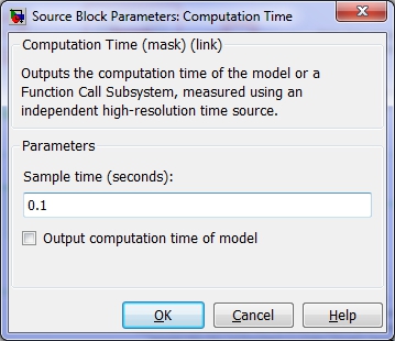
Its Sample time parameter is set to 0.1, so that the block executes in the slower rate task at 100 ms intervals. Note that QUARC supports any number of rates and is not limited to two tasks. Furthermore, each task is run in its own thread by default.
Blocks with a sample time of -1 inherit their sample time from their input signals. Most of the blocks in this model inherit their sample time.
In the slow rate task, this demonstration computes a matrix multiplication of two random 5x5 matrices and sums the matrix elements to produce a scalar output, as shown below:
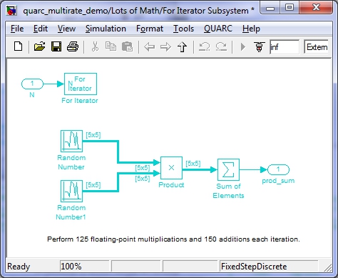
This computation is done inside a For Iterator Subsystem in which the number of iterations is controlled by an input port, N.
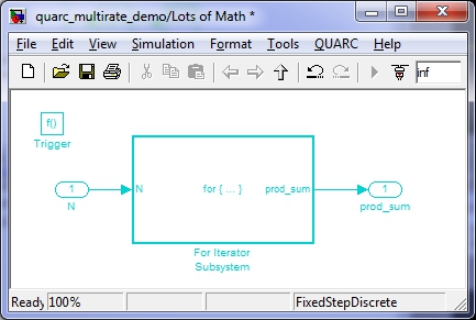
This entire computation is contained in the Lots of Math Function-Call Subsystem. This subsystem is invoked by the Computation Time block, which measures the time required to perform the entire computation.
The input N to the Lots of Math subsystem controls the number of iterations of the internal For Iterator Subsystem. By changing N, the number of computations can be modified.
One of the challenges in implementing this demonstration was ensuring that the computation time of the subrate task exceeded the base rate so that multiple threads were necessary to achieve proper sampling of both tasks. The ability to modify the number of computations performed by the Lots of Math subsystem provides the answer. The computation time of the subsystem is measured using the Computation Time block and then a proportional-integral (PI) controller is used to modulate the number of iterations, N, to achieve the desired computation time of 60 ms, independent of the speed of the target platform!
A desired computation time of 60 ms was chosen so that the fast rate task would need to execute at least six times during the computations done by the slow rate task.
In order to monitor the ability of QUARC to provide the desired sample rates, the sample times of the fast rate task and the slow rate task are measured using Sample Time blocks. Each Sample Time block is configured to run at the sample rate of the task whose rate they are measuring (see the Sample time parameter of each block).
The computation time of the Lots of Math subsystem is plotted in the Tc Scope. The number of iterations performed to achieve the desired 60 ms computation time is displayed in the N Display block on the diagram. The base-10 logarithm of N is traced in the log10(N) Scope in order to track of the output of the PI controller. A log plot is used because the value of N required to achieve 60 ms varies by orders of magnitude between QUARC targets.
The fast rate task produces a square wave via the Repeating Sequence Stair block that is plotted in the Fast Scope. The results of the Lots of Math computations in the slow rate task are displayed in the Slow Scope.
Configuring the Demonstration
To run the demonstration on the local Windows host no configuration should be required. The defaults should work.
Demonstration
This demonstration consists of two parts. First, the model is run in the default multi-tasking mode in which QUARC runs each task in its own thread. Then the configuration is changed to run in single-tasking mode so that the difference in performance may be observed. The multithreading capabilities of QUARC are a key differentiating factor between QUARC and inferior real-time products.
Running in Multi-Tasking Mode
Open the Configuration Parameters dialog by selecting from the menu, or by pressing Ctrl+E. Then navigate to the Solver pane in the Select treeview.
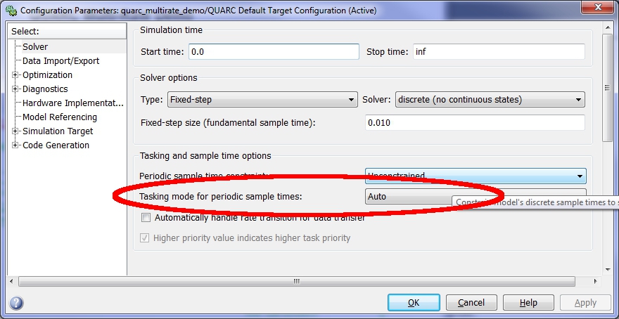
Make sure that the Tasking mode for periodic sample times parameter is set to or . The automatic setting chooses the appropriate tasking mode based on the number of sample times in the model. Since this example has multiple discrete rates it chooses the multi-tasking mode by default. Close the configuration dialog by clicking .
Select from the menu of the diagram, or press Ctrl+B while the diagram is the active window. A great deal of output will appear in the Diagnostic Viewer about the progress of the build. If you cannot see the Diagnostic Viewer, you can open it by selecting from the menu of the diagram, or clicking on the View Diagnostics hyperlink at the bottom of the diagram. If you have MATLAB R2013b or earlier then the output will appear in the MATLAB Command Window.
Double-click on the six Scope blocks in the diagram to display all the information about the model and its tasks.
Click on the button or select from the menu of the diagram to connect to the model.
Start the model by clicking on the button or selecting from the menu of the diagram. The item of the menu may also be used to both connect and start the model in one operation.
The Fast Scope will display a square wave with a 20 ms period, since the fast rate changes this output at its 10 ms sample time.
The Slow Scope shows a random value that varies approximately between -120 and 120. This value is the result of the Lots of Math computations in the slow rate task. Notice that the value changes every 100 ms or 0.1 seconds, since that is the sample time of the slow rate task.
The sample time of the fast rate task is depicted in the Fast Ts Scope. Notice that the sample time is a solid 10 ms or 0.01 seconds as desired.
The sample time of the slow rate task is shown in the Slow Ts Scope. Notice that the sample time is a solid 100 ms or 0.1 seconds as desired.
The Tc and log10(N) Scopes may initially display plots similar to the ones below:
Both plots are ramping up as the PI Controller increases the number of iterations in the Lots of Math subsystem in order to achieve the 60 ms computation time. It operates slowly because the gains are designed to work on all QUARC Targets, including embedded targets such as the gumstix Verdex, whose computational ability is orders of magnitude smaller than the latest Intel desktop processors.
If the model is left to run for a couple of minutes then the computation time, Tc, will eventually reach the 60 ms target, as depicted below:
Both plots have leveled off and the computation time is now the desired value. The number of iterations in this particular instance is 30487 iterations, as seen in the Display block:
Click on the button or select from the menu of the diagram to stop the model. The item of the menu may also be used.
Bear in mind that while these computations are being performed, the fast rate task has executed six times and yet both the fast and slow tasks have maintained their desired sample times of 0.01 seconds and 0.1 seconds respectively. The ability of QUARC to separate each task into its own thread is key to this performance.
To prove this assertion, consider what happens if QUARC is forced to generate a single thread that executes both the fast rate and slow rate tasks.
Running in Single-Tasking Mode
If QUARC is forced to run the model as a single task, then it will execute the fast rate ten times and then execute the slow rate once, repeatedly and sequentially. Since the slow rate task takes 60 ms to perform its computations, the fast rate task will not be able to execute at the desired rate of 10 ms whenever the slow task is run. This severe performance degradation will be observed in the Fast Ts Scope, which will show that the desired base rate is not being maintained.
To force the model to run as a single thread, open the Configuration Parameters dialog by selecting from the menu, or by pressing Ctrl+E. Then navigate to the Solver pane in the Select treeview.
Notice that the Tasking mode for periodic sample times parameter is set to . The automatic setting chooses the appropriate tasking mode based on the number of sample times in the model. Since this example has multiple discrete rates it chooses the multi-tasking mode by default.
Change the tasking mode to , as depicted below:
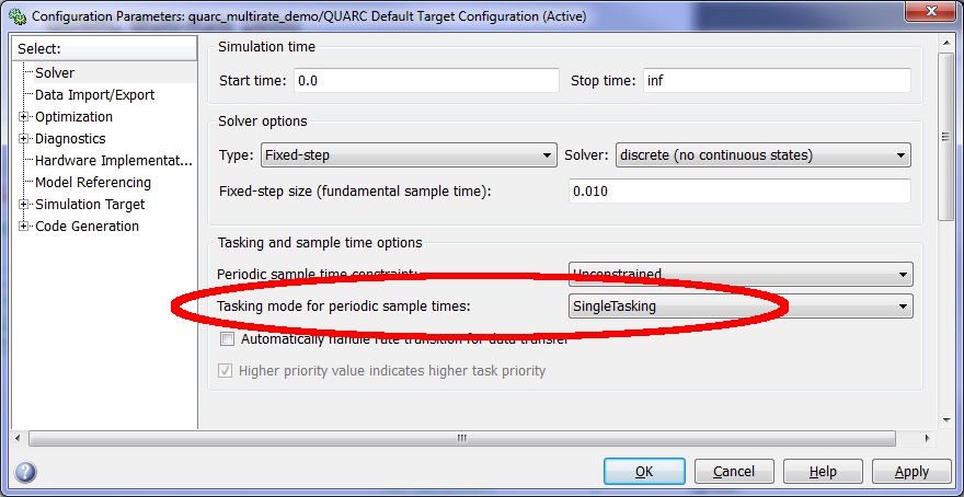
Using the SingleTasking mode forces QUARC to execute the model in a single thread. Close the configuration dialog by clicking . Now rebuild the model and run it again as follows.
Select from the menu of the diagram, or press Ctrl+B while the diagram is the active window. A great deal of output will appear in the Diagnostic Viewer about the progress of the build. If you cannot see the Diagnostic Viewer, you can open it by selecting from the menu of the diagram, or clicking on the View Diagnostics hyperlink at the bottom of the diagram. If you have MATLAB R2013b or earlier then the output will appear in the MATLAB Command Window.
Double-click on the six Scope blocks in the diagram to display all the information about the model and its tasks.
Click on the button or select from the menu of the diagram to connect to the model.
Start the model by clicking on the button or selecting from the menu of the diagram. The item of the menu may also be used to both connect and start the model in one operation.
If the target on which the model is being run is fast enough, it will actually be possible to see the threshold at which the single-tasking mode begins to break down and cannot provide the performance of the default multithreaded multi-tasking mode provided by QUARC.
The plots below depict the sampling rate of the fast task, Fast Ts, in single-tasking mode, as well as the sampling rate of the slow task, Slow Ts, and the computation time, Tc, as the PI controller ramps up the number of computations to try to achieve a 60 ms computation time. If it all happens too fast then consider reducing the Kp and Ki gains in the model so that the response is slower. Set the Kp gain to zero first as it is responsible for the initial jump in the number of computations.

Observe that the computation time in the plot starts around 0.01 seconds or 10 ms - the same interval as the fast rate task. As long as the computation time of the fast rate task combined with the slow rate task is less than the 10 ms then a single thread can provide the required base rate sample time. The plots above show what happens as the computation time of the slow rate task steadily increases beyond that threshold. The sample time of the base rate task starts to degrade because there is only a single thread of execution and the computations are taking more time than the required 10 ms sampling time.
The following graphs show a clearer picture of what is happening. The Fast Ts Scope and Tc Scope were auto-scaled to include the entire 20 seconds that the example had been running.
In the first 10 seconds or so of operation, the computation time, Tc, of the slow rate task was less 0.01 seconds or 10 ms. In those first 10 seconds the fast rate sample time of 0.01 seconds is maintained, as seen in the Fast Ts plot.
However, once the computation time, Tc, exceeds the 0.01 seconds at around a time of 10 seconds, the fast rate sampling time degrades proportionally, rapidly becoming worse.
A more detailed picture of what is transpiring is depicted in the Fast Ts plot below, in which the graph as magnified around the 18 second mark.
Notice that there is an upward spike every 0.1 seconds followed by an equal downward spike in the fast sample time. In between those spikes the desired 0.01 second sample time is maintained. This graph can be explained as follows. To execute the fast rate and slow rate tasks in a single thread, QUARC must execute the fast rate task nine times at the 0.01 second rate. At the tenth sampling instant, it must execute both the fast rate task and the slow rate task. It then repeats that sequence. This procedure results in the fast rate task executing every 0.01 seconds, and the slow rate task executing every 0.1 seconds - ten times slower, as desired. However, this scheme only works if the computation time of the fast and slow rate tasks combined is less than 0.01 seconds, which is not the case in this example.
So the flat portion of the graph that is level at 0.01 seconds is eight iterations when only the fast rate task is being executed.
The upward spike occurs because it is the tenth sampling instant and QUARC must execute both the fast rate task and the slow rate task. The slow rate task has a computation time of approximately 17 ms at that point. Since the computation time of the fast rate task in this case is negligible, the combined computation time is around 17 ms. Hence, the sample time jumps up to 17 ms as seen in the plot.
When the slow rate task has finished its computations, QUARC notices that the time at which it should have executed the fast rate task has already expired. Hence, it executes the fast rate code immediately. The next fast rate sampling instant occurs when it should, so the time between these two sampling instants is shorter. In fact, it is shorter by the difference between the computation time of the slow rate task and 0.01 seconds (10 ms), or a difference of about 7 ms. Hence, the measured sample time of the sample after the upward spike is only 10 - 7 = 3 ms.
After the shorter sampling period the thread is back in synchronization so the next eight sampling instants go at the required rate.
Click on the button or select from the menu of the diagram to stop the model. The item of the menu may also be used.
Do not forget to set the Tasking mode for periodic sample times parameter back to before saving the example model.
Clearly, the multithreading capabilities of QUARC are crucial to the performance of multi-rate control systems and are a significant advantage over competitive products that do not have such support. For more details of QUARC's multi-rate capabilities and additional features such as multi-core support, CPU affinities and Asynchronous Threads that are not covered in this demonstration, please refer to the Multithreading page in the QUARC documentation. On QNX targets, there are even more specialized scheduling features available with QUARC, such as bound multiprocessing and partition scheduling.
Running the example on a different target
To run the example on a different target, refer to the instructions on the Running QUARC Examples on Remote Targets page.
Copyright ©2026 Quanser Inc. This page was generated 2026-05-13. Submit feedback to Quanser about this page.
Link to this page.