
Polar Figure
Plots a polar graph in a separate window or on axes within a Matlab GUI.
Library
QUARC Targets/Sinks/Figures MATLAB Command Line Click to copy the following command line to the clipboard. Then paste it in the MATLAB Command Window: qc_open_library('quarc_library/Sinks/Figures')
Description

The Polar Figure block plots its rho and theta inputs on a polar graph. The Figure mode parameter determines where the plot is rendered. If both rho and theta are vectors (of the same dimensions) then it will plot one trace for each element of the inputs when the plotting mode is . If the plotting mode is then it will treat the rho and theta vectors as the points of a single curve.
If the figure mode is "Use figure window" then the plot is rendered in a separate window. In this case, the plot is opened by double-clicking on the block, just like a regular Scope. The properties of the block are accessed by clicking on the button on the toolbar or by right-clicking on the plot axes and selecting from the context menu. The help for the block is also accessible from a toolbar button and the context menu.
If the figure mode is "Use axes in GUI" then the plot is rendered on the axes of a preexisting MATLAB GUI. The GUI and axes are identified by the tag name associated with the figure and the axes. For example, a GUI created with GUIDE will have a tag name of 'figure1' and the first axes control placed in the GUI will have a tag name of 'axes1'. In this mode, double-clicking on the block will bring the GUI window forward if it is open, and add a context menu to the plot axes in the GUI. Otherwise it opens the block properties dialog. To access the properties of the block from the axes on the MATLAB GUI, right-click on the plot axes and select from the context menu. The help for the block is also accessible from this context menu. Note that the context menu is not available until either starting the model or double-clicking on the Polar Figure block.
The Polar Figure is available in the Signal & Scope Manager and External Mode Control Panel just like a Scope. As such, it may be used as a Viewer and it responds to the same triggering options as Scopes.
In the time-based plotting mode, the Polar Figure block buffers its input data in a circular buffer, which are plotted at periodic intervals. The size of the circular buffer may be specified via the Buffer size parameter. Since all the data in the circular buffer are plotted, making the buffer too large will compromise the performance of the plot.
The plotting interval is determined by the Update rate parameter, which is the number of samples that will be buffered before the plot is redrawn. For example, if the inputs to the block are 1kHz signals and the buffer size is 1000, then the plot will buffer the most recent 1 second worth of data in its circular buffer. If the update rate is set to 100 samples then the plot will draw the latest 1 second worth of data every 1/10th of a second (0.001 seconds * 100 samples), resulting in a relatively smooth plot with good performance. Making the update rate too small results in more plotting than necessary and the plot may fail to keep up with the data arriving at its inputs. If a very large number of points need to be plotted consider changing to a slower sample time for the plot in order to decimate the input signals.
The Polar Figure block also provides a toolbar button and context menu to autoscale the plot to the fit the current data. Simply click on the button in the figure window or select the menu item available in the context menu opened by right-clicking on the plot axes.
To access the help for the block, click on the button in the figure window or select the menu item available in the context menu opened by right-clicking on the plot axes.
Limitations
AppDesigner
 The Polar Figure block may not be used to create a polar plot on axes in an AppDesigner GUI because the axes
objects in AppDesigner GUIs do not support polar plots. However, it can be used to drive axes in a GUIDE GUI.
The Polar Figure block may not be used to create a polar plot on axes in an AppDesigner GUI because the axes
objects in AppDesigner GUIs do not support polar plots. However, it can be used to drive axes in a GUIDE GUI.
Input Ports
rho
The radius coordinate of the data to be plotted. This input may be a vector or scalar. If it is a vector then the theta input must have the same dimension.
theta
The angle coordinate of the data to be plotted, in radians. This input may be a vector or scalar. If it is a vector then the rho input must have the same dimension.
Output Ports
This block has no output ports.
Data Type Support
The Polar Figure block accepts signals of any of the built-in Simulink data types. Fixed point is not supported. Variable-size signals are supported at the inputs when the Plotting mode is frame-based.
Parameters and Dialog Box
Individual Panes
Main Pane
The Main pane of the dialog appears as follows:
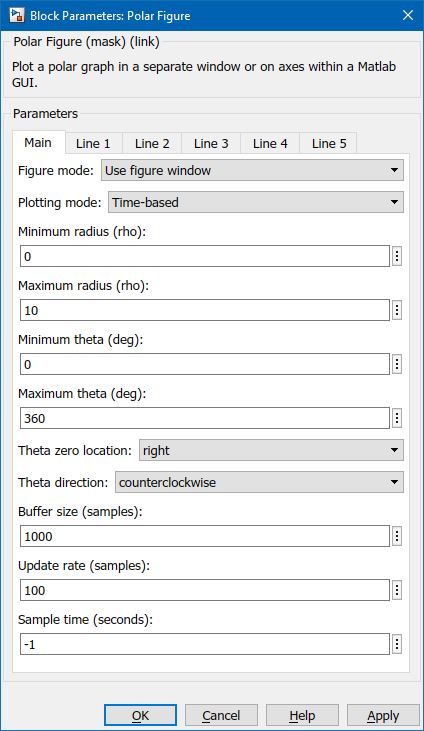
Figure mode
The figure mode determines whether the plot is rendered in a separate figure window or whether it is rendered on a set of axes contained within a MATLAB GUI. See the Description above for details.
Figure tag
This parameter is only visible when the figure mode is "Use axes in GUI". It identifies the MATLAB GUI in which the plot axes are contained by its tag name. The tag name may be changed in GUIDE by clicking on the background of the figure and then opening the Properties window. Scroll down to the "Tag" property in the Properties window. The default tag for figures is "figure1".
Axes tag
This parameter is only visible when the figure mode is "Use axes in GUI". It identifies the axes on which to plot by the tag name of the axes object. The tag name may be changed in GUIDE by clicking on the axes and then opening the Properties window. Scroll down to the "Tag" property in the Properties window. The default tag for the first axes control in the figure is "axes1".
Plotting mode
Chooses whether to treat the x and y inputs as individual points that are plotted as multiple curves over time or whether to treat the x and y inputs as the points of a single curve or frame to be plotted immediately. In the time-based mode, N-vector inputs are plotted as N distinct curves over time. In the frame-based mode, N-vector inputs are treated as N points on a single curve.
Minimum radius (rho)
The minimum value of the radius for the plot. Plot axes are fixed rather than autoscaling. This parameter is not available prior to MATLAB R2016a.
Maximum radius (rho)
The maximum value of the radius for the plot. Plot axes are fixed rather than autoscaling.
Minimum theta (deg)
The minimum value of the angle for the plot, in degrees. Plot axes are fixed rather than autoscaling. This parameter is not available prior to MATLAB R2016a.
Maximum theta (deg)
The maximum value of the angle for the plot, in degrees. Plot axes are fixed rather than autoscaling. This parameter is not available prior to MATLAB R2016a.
Theta zero location
The location where theta is zero. Valid values are right, top, left or bottom, indicating where on the plot theta is zero. This parameter is not available prior to MATLAB R2016a.
Theta direction
Whether the angles increase in a counterclockwise direction or a clockwise direction. The default is counterclockwise.
Buffer size
This parameter determines the size of the circular buffer used by the plot, in samples. Making this parameter too large can compromise the performance of the plot. The default buffer size is 1000 samples.
Update rate (samples)
The update rate determines the frequency with which the plot is redrawn. Like the buffer size, it is specified in samples. The smaller this parameter the more frequently the plot is redrawn. The plot is redrawn every (update rate * sample time) seconds. Updating the plot faster than 1/10th of a second is generally unnecessary and is not recommended as it compromises the performance of the plot. However, note that all the samples collected in the circular buffer are still plotted. This parameter does not decimate the data - it only determines how often the plot is updated with the latest data.
Sample time
The sample time of the block. A sample time of 0 indicates that the block will be treated as a continuous time block. A positive sample time indicates that the block is a discrete time block with the given sample time.
A sample time of -1 indicates that the block inherits its sample time from the input. The block inherits the sample time by default.
To set the sample time to the fundamental sampling time of the model, use the qc_get_step_size function, which is a QUARC function that returns the fundamental sampling time of the model. The fundamental sampling time of the model is the sampling time entered in the Fixed step size field of the Solver pane of the Configuration parameters.
Line {x} Pane
The Line {x} pane of the dialog appears as follows:
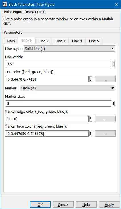
Line style
The style of line {x}.
Line width
The width of line {x].
Line color
The RGB colour value as a 3-vector for line {x}. Each element must lie in the range 0 to 1. The order of the elements is [red, green, blue]. Use the browse button next to this parameter to select a color using a color picker.
Marker
The marker to be used for line {x}.
Marker size
The size of the marker to be used for line {x}.
Marker edge color
The RGB colour value as a 3-vector for line {x}'s marker edge. Each element must lie in the range 0 to 1. The order of the elements is [red, green, blue]. Use the browse button next to this parameter to select a color using a color picker.
Marker face color
The RGB colour value as a 3-vector for line {x}'s marker face. Each element must lie in the range 0 to 1. The order of the elements is [red, green, blue]. Use the browse button next to this parameter to select a color using a color picker.
Targets
|
Target Name |
Compatible* |
Model Referencing |
Comments |
|---|---|---|---|
|
Yes |
Yes |
||
|
Yes |
Yes |
||
|
Yes |
Yes |
||
|
Yes |
Yes |
||
|
Yes |
Yes |
||
|
Yes |
Yes |
||
|
Yes |
Yes |
||
|
Yes |
Yes |
||
|
Yes |
Yes |
||
|
Yes |
Yes |
||
|
Yes |
Yes |
||
|
Yes |
Yes |
||
|
Yes |
Yes |
||
|
Yes |
Yes |
Last fully supported in QUARC 2018. |
|
|
Rapid Simulation (RSIM) Target |
Yes |
Yes |
|
|
S-Function Target |
No |
N/A |
Old technology. Use model referencing instead. |
|
Normal simulation |
Yes |
Yes |
See Also
Copyright ©2026 Quanser Inc. This page was generated 2026-05-13. Submit feedback to Quanser about this page.
Link to this page.