RCP CL Continuous Sigmoid Example

navigation bar

Table of Contents >Quanser Rapid Control Prototyping Toolkit >Examples >Basic Features >

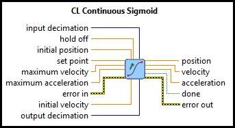
This example demonstrates how to use the RCP CL Continuous Sigmoid VI. For a detailed description of this VI and how it operates, please refer to the RCP CL Continuous Sigmoid help page.

System Requirements

Please refer to the Rapid Control Prototyping (RCP) Toolkit System Requirements to run this example. This example does not require any other hardware.

Configuring the Example

There is no configuration required to run this VI on a Windows PC. Once the RCP CL Continuous Sigmoid Example.lvproj is open, click the RCP CL Continuous Sigmoid Example.vi under My Computer and you are ready to execute the example.

Running the Example

Click on the VI Run button or select Run from the Operator menu to start the VI.

The Position chart shows the original square wave signal (blue) and the resulting smoothed trajectory generated by the sigmoid (red). The calculated velocity and acceleration of the trajectory are displayed in the Velocity and Acceleration scopes.

The Maximum Velocity and Maximum Acceleration parameters of the sigmoid impose limits on the generated trajectories. Try changing the parameters and examine their effect on the position, velocity, and acceleration trajectories.

Click on the Front Panel Stop button to stop the VI.

navigation bar